TLE Analysis
This analysis takes the Two-Line Element (TLE) of a satellite and an observer’s latitude and longitude to find the azimuth and elevation of the satellite from the observer’s point of view.
We start with the Keplerian elements, which are part of a TLE. They are a description of a satellite’s orbit and have to be updated every few days due to drag, gravitational pull from other bodies, and everything else that makes the situation not a simple two body problem. There are seven elements which can be found in bulletins in places like AmSat and CelesTrak. Inclination \((I_0)\), RAAN \((\Omega_0)\), and argument of perigee \((\omega_0)\) all define the specific angles of intersection between the orbital plane and the Earth. The mean motion \((N_0)\) is the average speed of the satellite and the eccentricity of the orbit \((e\)) determines how close it is to a perfect circle. The last two come as a pair and are epoch \((T_0)\) and mean anomaly \((M_0)\). The mean anomaly is an angle measured between the current position of the satellite and the perigee, while the epoch is the time at which this angle was recorded. (“Keplerian Elements Tutorial”)
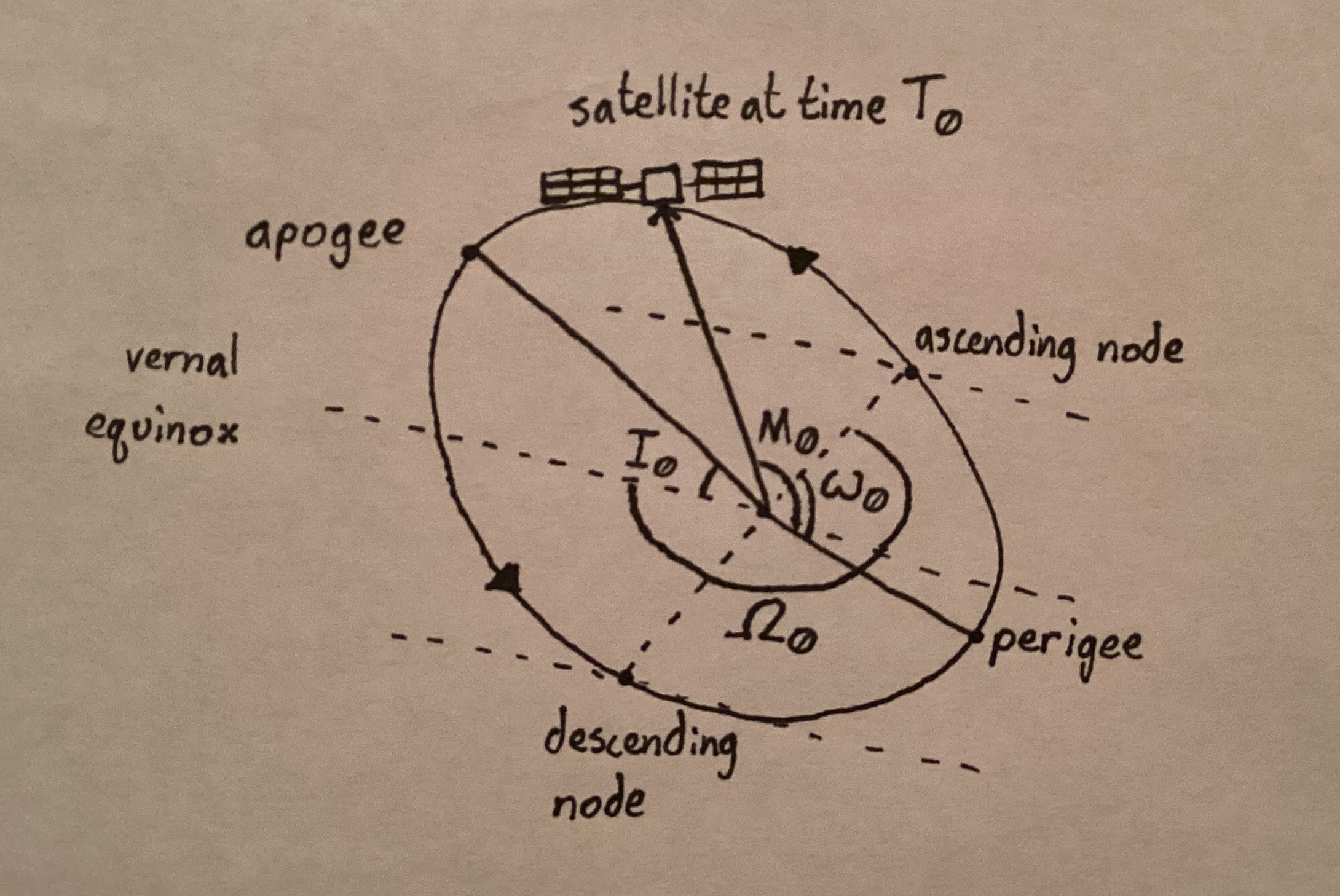
The first step to finding the satellite’s location is to find the angle it is currently at around its orbit. Using the mean motion, we can see how many radians around its orbit the satellite has traveled since its epoch (“Mean Anomaly”).
\[ M_f = M_0 + N_0(T_0 - T_f) \tag{1} \]Satellites’ orbits around Earth are not perfect circles, so we have to find the eccentric anomaly to adjust for this. To find the eccentric anomaly from the current anomaly, we have to do something called a Newton-Raphson estimation. The formula is as follows (Cybernetic Systems and Controls 27:26).
\[ E = \sum_{i=1}^{n} \left[E_{i-1} - \frac{M_f - E_{i-1} + e \cdot \sin(E_{i-1})}{e \cdot \cos(E_{i-1})-1}\right] \tag{2} \]I took \(E_0\) to be equal to \(M_f\) and continued the process five times, until the error was minor. Once we have the eccentric anomaly, we can find the true anomaly \((f)\) (Cybernetic Systems and Controls 0:50).
\[ tan \frac{f}{2} = tan \frac{E}{2} \sqrt{\frac{1+e}{1-e}} \tag{3} \]Now that we have the angle, we want to find how far away it is so we can put it into an XYZ coordinate system. To find the radius, we’ll first need to find the semi-major axis \((a)\). Kepler’s second law states (Nave):
\[ T^2 = \frac{4a^3\pi}{\mu} \tag{4} \]The period (\(T\)) is the mean motion \((N_0)\) and \(\mu\) is the standard gravitational parameter for Earth. Both of these are known, so we can solve for \(a\). Knowing the semi-major axis allows us to find the current distance from its center of orbit with the following (Still).
\[ r = a[1 - e \cdot \cos(E)] \tag{5} \]Now that we have the current radius, we can use this, the true anomaly, and the three orientation Keplerian elements to get the current position of the satellite in Earth-Centered Inertial (ECI) coordinates. We do this by turning the radius and anomaly into Perifocal coordinates and then multiplying by three rotation matrices, one for each Keplerian element (Peet 35). The expressions work out to
\[ X_{sat} = r\left[\cos(\Omega_0)\cos(\omega_0 + f) - \sin(\Omega_0)\sin(\omega_0 + f)\cos(I_0)\right] \tag{6} \]\[ Y_{sat} = r[\sin(\Omega_0)\cos(\omega_0 + f) + \cos(\Omega_0)\sin(\omega_0 + f)\cos(I_0)] \tag{7} \]
\[ Z_{sat} = r[\sin(\omega_0 + f)\sin(I_0)] \tag{8} \]
We can now focus on the Satellite Pointer’s position in space. We know its latitude \((\phi)\), longitude \((\lambda)\), and the current time \((T_f)\). The first step is to turn longitude and latitude into Earth-Centered Earth-Fixed (ECEF) coordinates. While this system does not account for rotation of the Earth, it is an XYZ system and shares an origin with ECI coordinates, getting us one step closer. The conversions are as follows (“From geodetic to ECEF coordinates”).
\[ X_{ECEF} = N_\phi \cos(\phi)\cos(\lambda) \tag{9} \]\[ Y_{ECEF} = N_\phi \cos(\phi)\sin(\lambda) \tag{10} \]\[ Z_{ECEF} = (1 - f_{Earth})^2N_\phi \sin(\phi) \tag{11} \]
We need to find the curvature in the prime vertical \((N_\phi)\) and the flattening factor \((f)\).The prime vertical is given by the following (“Prime Vertical”).
\[ N_\phi = \frac{a}{\sqrt{1 - e_{Earth}^2\sin^2(\phi)}} \tag{12} \]We can get \(N\) in terms of the flattening factor \((f)\) and the Earth’s semi-major axis \((a_{Earth})\).
\[ e^2 = 2f - f^2 \tag{13} \]\[ N_\phi = \frac{a}{\sqrt{1 - (2f - f^2)\sin^2(\phi)}} \tag{14} \]
Now the ECEF coordinates are in terms of the latitude, longitude, Earth’s semi-major axis, and Earth’s flattening factor. The latter two are known measured values part of a geodetic reference system. The most accurate model is GRS 80, which gives \(a_{Earth}\) as \(6,378,137\) meters and \(f\) as \(3.352811 \times 10^{-3}\) (“Geodetic Reference System 1980”).
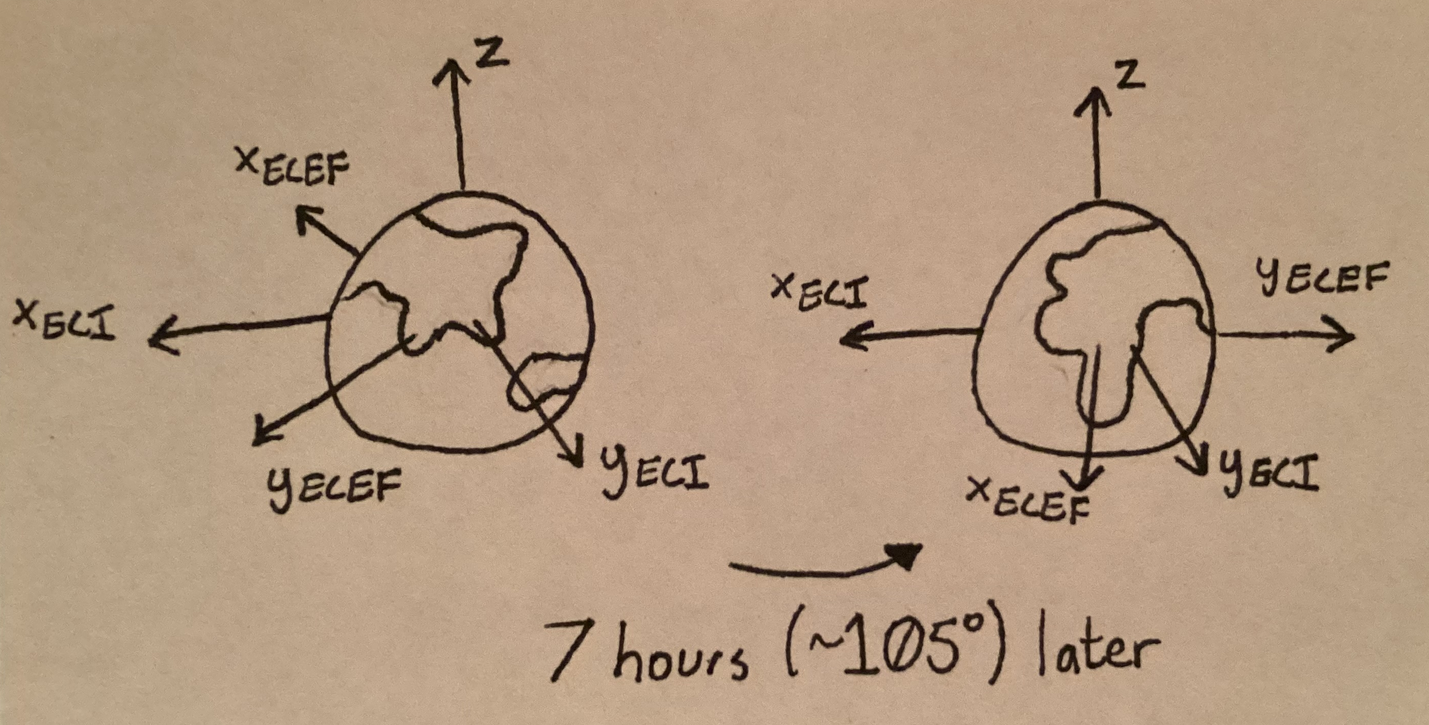
Now in ECEF coordinates, we need to get them to ECI coordinates to match the satellite position. They both share the same z-axis, but ECEF coordinates move with the Earth while ECI coordinates remain fixed. The conversion between the two involves a rotation matrix that uses the Greenwich sidereal angle \((\gamma)\) (Koks 29). This angle depends on a standard reference known as a Julian date. We can find the current Julian date \((JD)\) using this formula (Jefferys).
\[ JD = \lfloor 365.24(year + 4716) \rfloor + \lfloor 30.6001(month + 1) \rfloor + day + 2 - \lfloor \frac{year}{100} \rfloor + \lfloor 0.25 \lfloor \frac{year}{100} \rfloor \rfloor - 1524.5 \tag{15} \]From the Julian date \((JD)\), we can get the Greenwich angle (Still).
\[ \gamma = 280.46061837 + 360.98564736629(JD - 2451545) + 3.87933 \left(\frac{JD}{36525}\right)^2 10^{-4} - \left(\frac{JD}{36535}\right)^3 \frac{1}{38710000} \frac{\pi}{180} \tag{16} \]Multiplying the X and Y ECEF coordinates by this rotation matrix, we get
\[ X_{Earth} = X_{ECEF}\cos(\gamma) - Y_{ECEF}\sin(\gamma) \tag{17} \]\[ Y_{Earth} = X_{ECEF}\sin(\gamma) + Y_{ECEF}\cos(\gamma) \tag{18} \]
Remember they both share the same z-axis, so
\[ Z_{ECEF} = Z_{Earth} \tag{19} \]Now that we have two points in space, we can find the angles the vector between them makes with some vector analysis and linear algebra. The elevation is with respect to the tangent plane of the current position, so we first need to find an equation for that. We know its normal vector is
\[ \vec{n}_{pos} = \frac{1}{\sqrt{X_{Earth}^2 + Y_{Earth}^2 + Z_{Earth}^2}} \langle X_{Earth},Y_{Earth},Z_{Earth} \rangle \tag{20} \]The line of site (LOS) vector is the one we are measuring the angles of, which is given by
\[ \vec{v}_{LOS} = \langle X_{sat} - X_{Earth}, Y_{sat} - Y_{Earth}, Z_{sat} - Z_{Earth} \rangle \tag{21} \]We can find the angle between these two using
\[ \cos(\alpha) = \frac{\vec{n}_{pos} \cdot \vec{v}_{LOS}}{||\vec{v}_{LOS}||} \tag{22} \]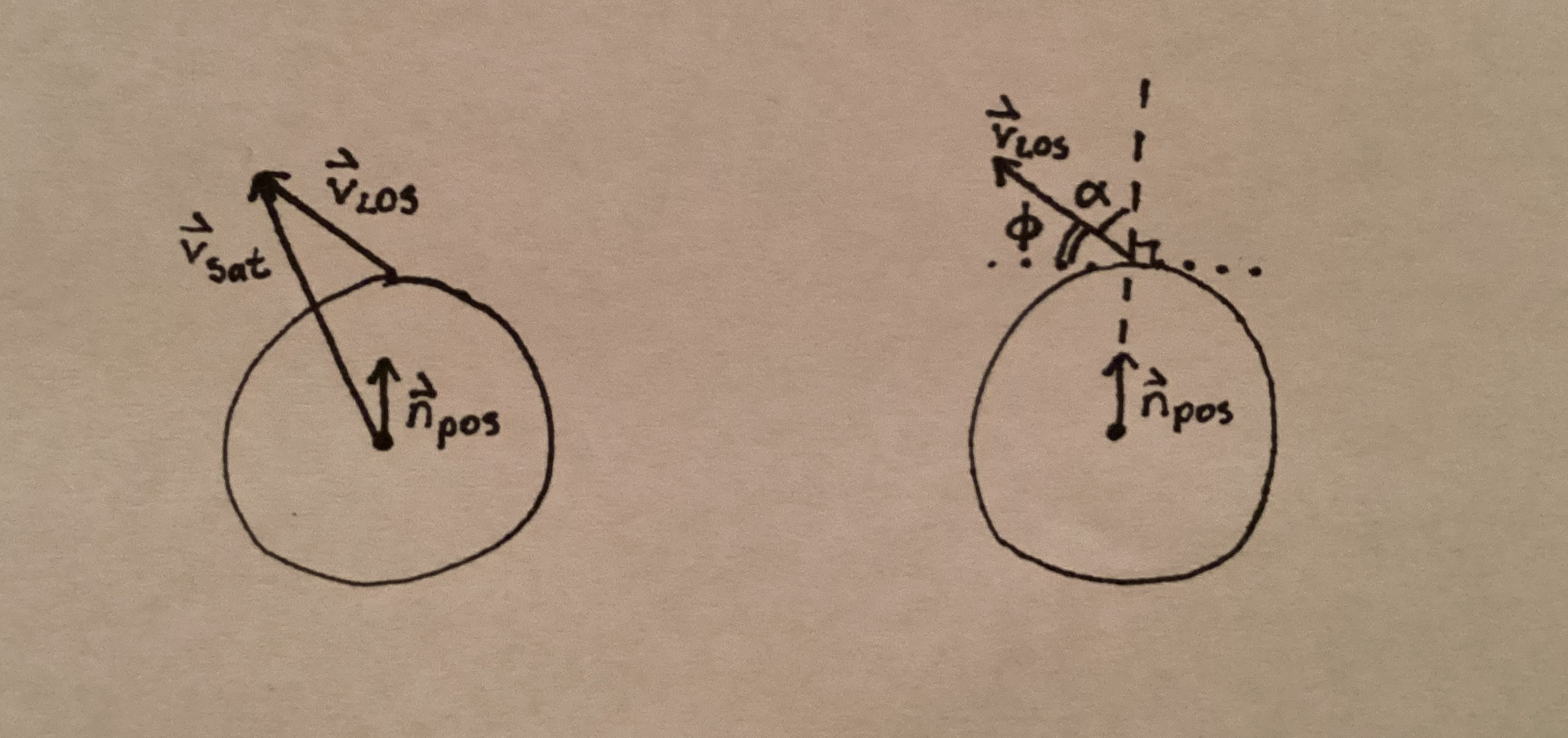
This will not turn out to be the elevation angle, as this angle is measured from straight up and down, not from the horizon. As the elevation equals \(\frac{\pi}{2}\) minus the equation above, we can take \(phi\) to be
\[ \phi = \sin^{-1}(\frac{\vec{n}_{pos} \cdot \vec{v}_{LOS}}{||\vec{v}_{LOS}||}) \tag{23} \]Azimuth is slightly harder to find as its reference point is North and it can be out of \(2\pi\) compared to \(\pi\). To get the correct azimuth, both North and West have to be defined.
\[ \vec{n}_{North} = \langle 0,0,1 \rangle \tag{24} \]\[ \vec{n}_{West} = \frac{\vec{n}_{pos} \times \vec{n}_{North}}{||\vec{n}_{pos} \times \vec{n}_{North}||} \tag{25} \]
To just focus on the azimuth, we need to flatten the line of sight vector onto the tangent plane of the location on Earth. This is done using
\[ \vec{v}_{flat} = \vec{n}_{LOS} - \frac{\vec{n}_{LOS} \cdot \vec{v}_{pos}}{||\vec{v}_{pos}||^2}\vec{v}_{pos} \tag{26} \]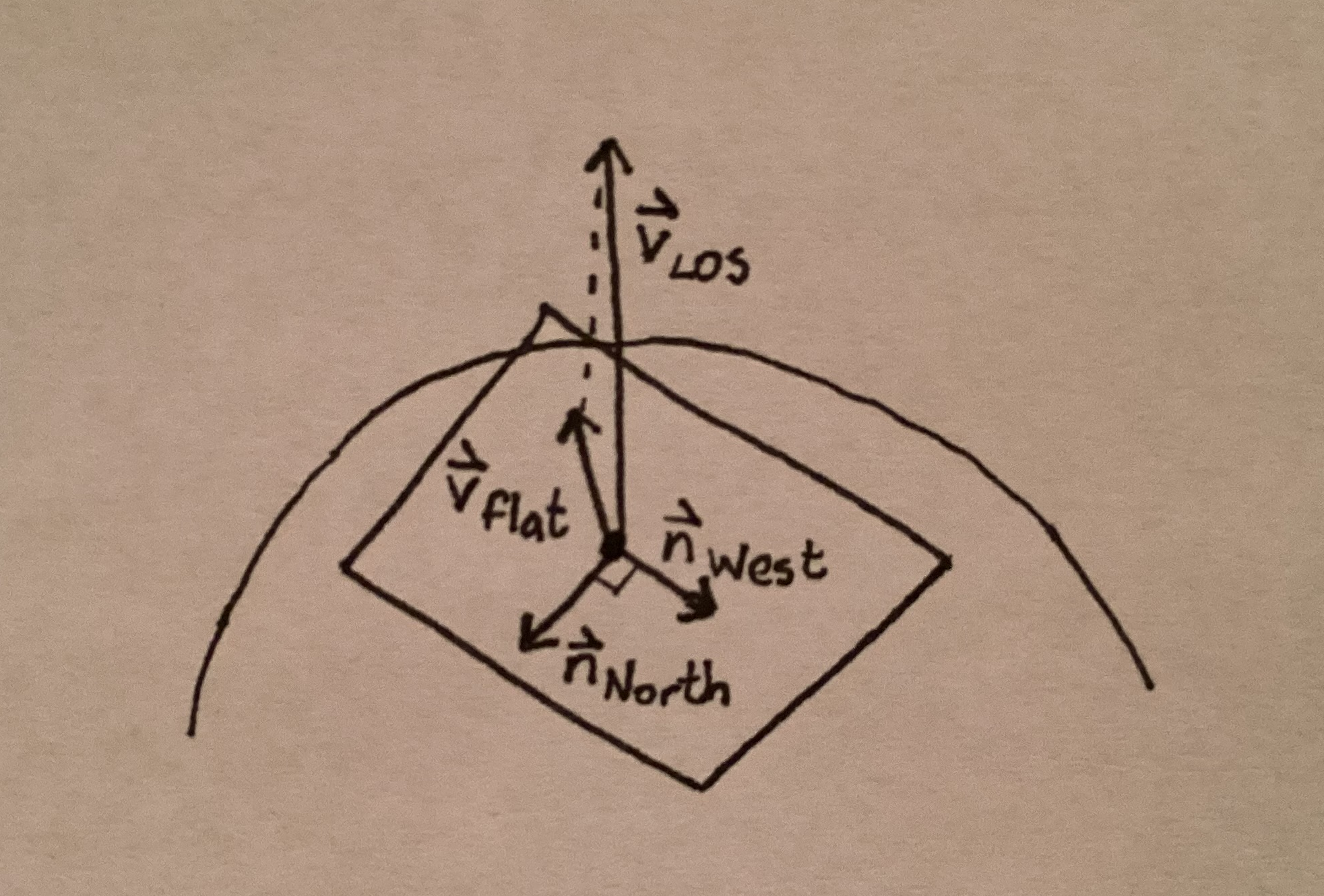
Now we can set up a dot product to find the angle. Using tangent instead of cosine allows us to find which quadrant the azimuth is in. We get the equation
\[ \theta = tan^{-1}(\vec{n}_{North} \cdot \vec{v}_{flat} - \vec{n}_{West} \cdot \vec{v}_{flat}) \tag{27} \]We now have both the azimuth \((\theta)\) and elevation \((\phi)\) needed to point at a satellite at any time from any location on Earth.
Sources Cited
Cybernetic Systems and Controls, “AEE462 Lecture 4, Part B - Newton-Raphson Iteration and Kepler’s Equation”, Youtube, 2 February 2021, https://www.youtube.com/watch?v=fqHdfJ7d7SY&t=19s Accessed June 11, 2026
“From geodetic to ECEF coordinates”. “Geographic coordinate conversion”, Wikipedia, The Free Encyclopedia, Wikimedia Foundation, 18 May 2026, https://en.wikipedia.org/wiki/Geographic_coordinate_conversion#From_geodetic_to_ECEF_coordinates Accessed June 11, 2026
“Geodetic Reference System 1980”. Wikipedia, The Free Encyclopedia, Wikimedia Foundation, 13 November 2025, https://en.wikipedia.org/wiki/Geodetic_Reference_System_1980 Accessed August 31, 2026
Jefferys, William. “Julian Day Numbers”, University of Texas at Austin, 1998, https://quasar.as.utexas.edu/BillInfo/JulianDatesG.html Accessed June 11, 2026
“Keplerian Elements Tutorial”. AmSat, 2026, https://www.amsat.org/keplerian-elements-tutorial/ Accessed June 11, 2026
Koks, Don. “Changing Coordinates in the Context of Orbital Mechanics”, Australian Department of Defense Science and Technology, Cyber and Electronic Warfare Division, January 2017, https://apps.dtic.mil/sti/tr/pdf/AD1027338.pdf Accessed June 11, 2026
“Mean Anomaly”. Wikipedia, The Free Encyclopedia, Wikimedia Foundation, 14 May 2026, https://en.wikipedia.org/wiki/Mean_anomaly Accessed June 11, 2026
Nave, R. “The Law of Periods”, HyperPhysics, http://hyperphysics.phy-astr.gsu.edu/hbase/kepler.html Accessed June 11, 2026
Peet, Matthew. “Spacecraft Dynamics and Control Lecture 7: Converting to/from r and v”, Arizona State University, https://control.asu.edu/Classes/MAE462/462Lecture07.pdf Accessed June 11, 2026
“Prime vertical”, “Earth Radius”. Wikipedia, The Free Encyclopedia, Wikimedia Foundation, 24 July 2026, https://en.wikipedia.org/wiki/Earth_radius#Prime_vertical Accessed August 31, 2026
Still, James. “Kepler’s Equation”, Square Widget, 9 April 2019, https://squarewidget.com/keplers-equation/ Accessed June 11, 2026
Still, James. “Sidereal Time”, Square Widget, 9 April, 2019, https://squarewidget.com/astronomical-calculations-sidereal-time/ Accessed June 11, 2026